This was a case study on one of the client projects that I was involved with at Cape AI.

Introduction

We recently completed a computer vision project for a client in the Agritech sector, Arcitechnologies. At Cape AI, we’re always excited to work on a project involving deep learning. In particular, we love working on challenging computer vision projects which allow us to leverage cutting edge techniques to solve modern problems. In this post, we will discuss the problem, our approach to solving it, and share additional insights and lessons learnt in creating lasting value through deep learning.

The Use Case

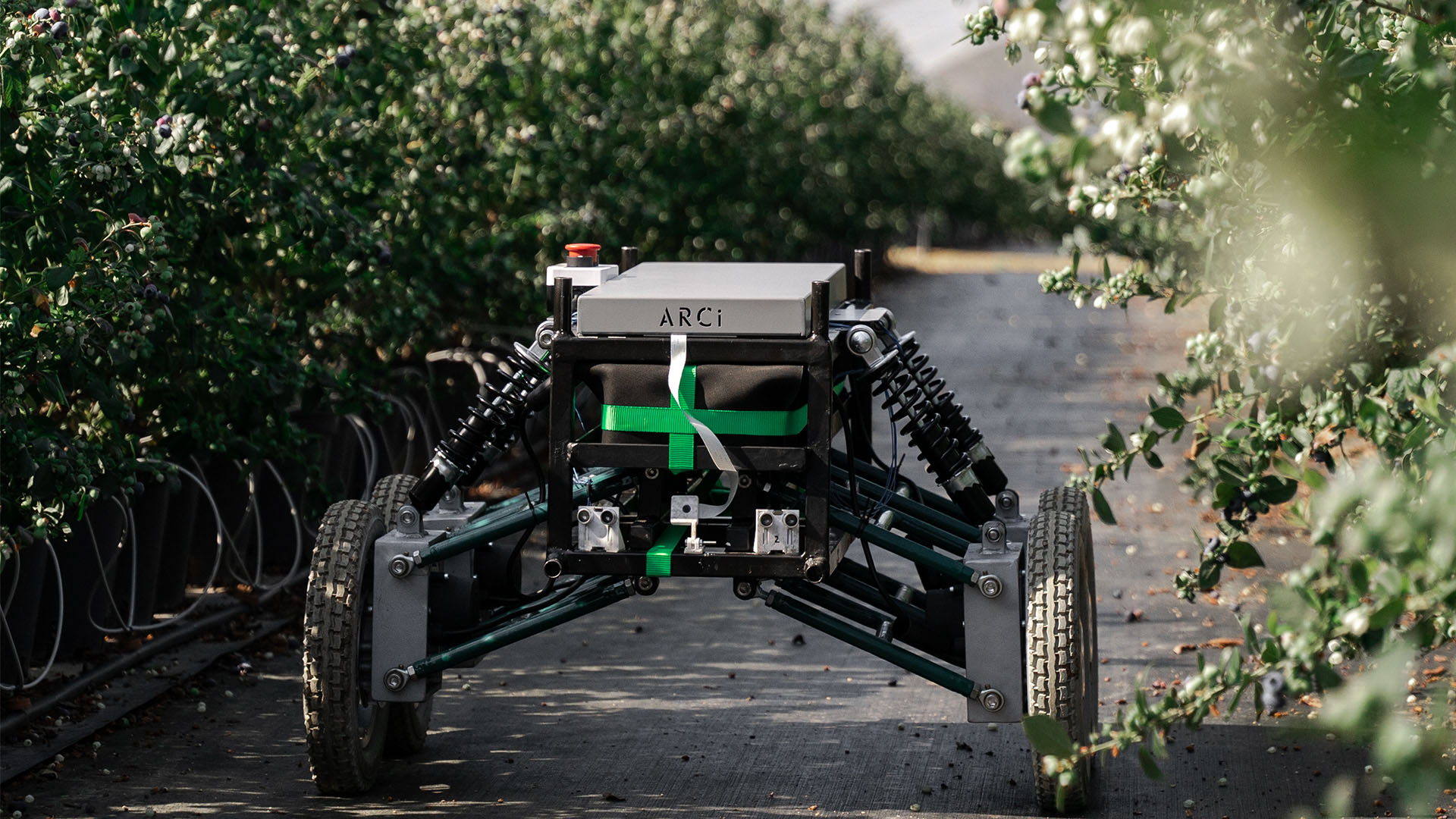
Arcitechnologies is a technology startup based in Stellenbosch, South Africa, that is innovating in the Agricultural sector. They're doing this by building a semi-autonomous robot which can provide support to workers on blueberry farms in Stellenbosch, and also provide harvest predictions to farmers to help them manage their business.

The robot needs to navigate a variety of non-uniform environments and therefore needs to be enabled with the right tools to identify objects in its environment and navigate safely in real-time with no human input.

To achieve this, the client needed a model which could identify where the robot could safely drive without harming itself, crops or human workers.

Cue AI and computer vision!

Our Approach

The key whenever approaching a business problem is understanding the customer's needs, requirements, and their context. Our initial engagements with the client highlighted that the robot will have a fully mounted computer onboard as well as cameras on the front. With this in mind, we decided that deploying a model to run on the device and integrating the model outputs with the navigation system would be best. In addition, the client also asked that we engineer a simple model pipeline which would allow them to easily integrate models of their own in the future.

After establishing the client's needs and context, we began an exploratory exercise to determine what model would be best suited to solving this kind of problem. We settled on a semantic segmentation model for this problem. This is because in the field of automated navigation, semantic segmentation is often used for creating a nuanced understanding of the environment for the agent. For example, companies such as Tesla, Google and Toyota and others pursuing autonomous vehicles use semantic segmentation as the backbone of their navigation systems.

Modeling

Navigation use cases are tricky. This is because tiny details in images can have a significant influence on navigation accuracy. Semantic segmentation models work by classifying every pixel in an image, thereby giving attention to the tiny details needed to solve navigation problems. By knowing exactly where an obstacle begins and ends, we can give the robot the best chance of making the correct decisions on where it needs to go.

To train this model we needed a dataset of images and semantic masks from the environment that the robot would eventually be deployed in, namely the rows of blueberry bushes from the farm. Luckily, our client already had a fair amount of footage gathered from the robot, so all that needed to be done was to label this data.

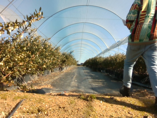
Just a normal day on the farm

We then created a dataset composed of five classes:

• Person
• Gravel
• Weed-mat
• Grass
• Non-traversable.

By breaking down what the model would identify into these pieces we could get a fairly fine-grain understanding of what was in front of the robot. This would allow the robot to determine how to avoid driving into the bushes next to it, to identify traversable ground, and to know when it had reached the end of a row.

The client outsourced the data-labeling for this project and soon thereafter we had a reasonably high-quality but small dataset that we could import into CVAT, our data labeling tool of choice. CVAT allowed us to export our data to any data format we wanted. This gave us flexibility when creating our model training pipeline as we were not confined to only one data format.

Building the model

Now that we had our data it was time to get started with building the model. For this we used the segmentation models library which is a high level API built on top of the pytorch deep-learning framework. This significantly speeds up development as it allows you to pull architectures from a remote repository and create a model with very few lines of code.

Here is a template of the notebook we ended up using for model training if you'd like to experiment on this kind of problem. Feel free to try it out on a sample dataset of your own!

For this project we primarily worked in Google Colab, taking advantage of the free GPU and built-in libraries. We chose Colab because it provides a great environment for learning due to their nature as a live coding environment where you have direct access to variables at all times and can see how the code works at each step. This lets you see what the code is doing piece by piece and let's you experiment with it as you go, which would help Arcitechnologies to understand and use the code themselves in future.

Preparing the data

After we'd done our imports and installed the packages we wanted to use we began with data preparation.

In our case, we did not have a large amount of data at our disposal, around 350 images, so we planned to simply do some fine-tuning on a pre-trained model to take advantage of what the model has already learned.

In handling the data and exporting it from CVAT, we chose the CAMVID data format so as to match the dataloaders we were using. It helped to split the data before bringing it onto the notebook by using the split-folders python library. This made it easy to create a simple folder structure which we could then upload to cloud storage, in this case Google Drive, and then import into our notebook.

Extracting the annotation data from the masks

In training semantic segmentation models, masks are used as a way of encoding where a certain type of entity exists in an image. In the example below the mask is indicating the areas of the image where there is a human in red, non-traversable terrain in very dark green, and grass in lighter green.

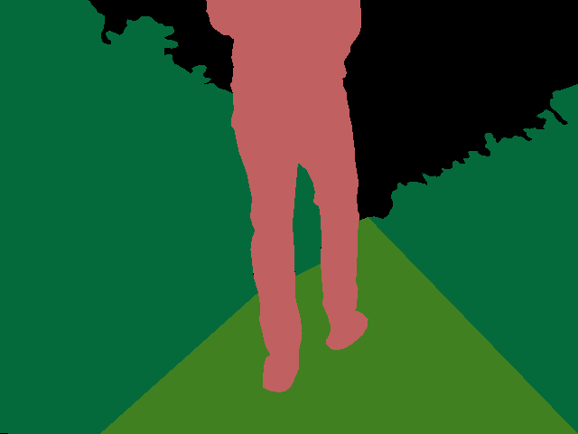
One challenge which we faced in solving this problem was figuring out how to programmatically identify which colour region mapped to each class. While this is very easy with the eye it is difficult to code a way to do it without a clear mapping of colour to class. Luckily, we eventually found a file that shipped with the dataset that matched each label to each colour in the masks. Now all we needed to do was turn our raw data into a pytorch dataset.

Loading the data into a pytorch dataset

At this point we had a bunch of folders with our images and masks. Our next step was to create a dataset object which could hold references to these masks and images and also perform pre-processing and augmentation operations on these images so that we could train on them.

To do that, we created a dataset class which allowed us to quickly perform augmentation and pre-processing operations on our data.

At this point, we were now able to generate the figure below. This figure shows a sample of the raw image data and its corresponding mask. As you can see, there is a rock on the ground that has been labeled as non-traversable terrain which may later be useful in the robot's decision making.

Data augmentation and preprocessing

The next step was to apply pre-processing and augmentations to the data so that we could create diversity in the data, and to normalise the data for our selected model architecture. Data normalisation is helpful because it helps us to create a smoother gradient descent in our model's learning. Without this step it is likely that our model will train much more slowly, as the inputs would generally be outside of the range that the model expects for training.

We specifically use pre-processing that is designed for our model's architecture, as different encoders have differences in the values that they expect.

We also apply some standard data augmentation steps to the dataset which help it avoid overfitting to the training data and become more generalisable. Some examples of the kind of augmentation we used were things like:

• Altering the hues, brightness and contrast in an image. This produces the dark red on the bushes as you can see below.
• Zooming in on a portion of the image.
• Rotating the image. This is critical because the robot will often not be perfectly horizontal.
• Adding noise and blur to the image.

The results are shown below:

Defining the model

Here we leverage the segmentation models library to instantiate our model with the parameters we want.

ENCODER = 'se_resnext50_32x4d'
ENCODER_WEIGHTS = 'imagenet'
CLASSES = CLASSES
ACTIVATION = 'sigmoid' 
DEVICE = 'cuda'

# create segmentation model with pretrained encoder
model = segmentation_models_pytorch.FPN(
    encoder_name=ENCODER, 
    encoder_weights=ENCODER_WEIGHTS, 
    classes=len(CLASSES), 
    activation=ACTIVATION,
)

#downloading the default model weights can take some time, normally ~5 minutes

preprocessing_fn = smp.encoders.get_preprocessing_fn(ENCODER, ENCODER_WEIGHTS)

We chose to use resnext50 for its high accuracy and relatively fast inference speed. If you're interested, there is a wide selection of models available to use. Check it out on the github page.

We then used the segmentation models library to create and build the model using our predefined parameters.

Model training

To begin training we must load our data into the training pipeline.

For this we needed to create training and validation datasets and then create runners which would go back and forth to fetch samples and pass them into the model.

#Here we create our validation and training datasets and apply augmentation and preprocessing

train_dataset = Dataset(
    x_train_dir, 
    y_train_dir, 
    augmentation=get_training_augmentation(), 
    preprocessing=get_preprocessing(preprocessing_fn),
    classes=CLASSES,
)

valid_dataset = Dataset(
    x_valid_dir, 
    y_valid_dir, 
    augmentation=get_validation_augmentation(), 
    preprocessing=get_preprocessing(preprocessing_fn),
    classes=CLASSES,
)

train_loader = DataLoader(train_dataset, batch_size=8, shuffle=True, num_workers=12)
valid_loader = DataLoader(valid_dataset, batch_size=1, shuffle=False, num_workers=4)

We used the Pytorch dataloader object to pass in our datasets. Depending on the amount of memory on our GPU, this occasionally needed to be adjusted on our train_loader. Normally, an even number between 4 and 16 would be a decent choice for this kind of dataset.

We then chose our loss function and optimizer, in this case dice loss and Adam respectively. These are both tried and tested parameters and allow for rapid model training.

The rest of the process involved creating epoch runners and iterating over our samples.

# train model for 40 epochs

max_score = 0

for i in range(0, 40):
    print('\nEpoch: {}'.format(i))
    train_logs = train_epoch.run(train_loader)
    valid_logs = valid_epoch.run(valid_loader)
    
    # do something (save model, change lr, etc.)
    if max_score < valid_logs['iou_score']:
        max_score = valid_logs['iou_score']
        torch.save(model, './best_model_5_classes.pth')
        
        print('Model saved!')
        
    if i == 25:
        optimizer.param_groups[0]['lr'] = 1e-5
        print('Decrease decoder learning rate to 1e-5!')

We trained for 40 epochs taking approximately 40 to 50 minutes to complete. If this seems fast, keep in mind that we are leveraging transfer learning of a model that has been trained for much longer, and we are also using a really good optimizer in Adam to quickly get to great performance. It is also quite a small dataset.

Evaluating the results

To evaluate our model's performance, we created a test dataset, an epoch runner to go with it, and applied our trained model on the test set.

# create test dataset
test_dataset = Dataset(
    x_test_dir, 
    y_test_dir, 
    augmentation=get_validation_augmentation(), 
    preprocessing=get_preprocessing(preprocessing_fn),
    classes=CLASSES,
)

test_dataloader = DataLoader(test_dataset)

# evaluate model on test set
test_epoch = smp.utils.train.ValidEpoch(
    model=best_model,
    loss=loss,
    metrics=metrics,
    device=DEVICE,
)

logs = test_epoch.run(test_dataloader)

After running this we achieved a performance of approximately 93% IOU (Intersection Over Union). This is an estimation of how much the model's prediction overlapped with the ground truth. This is a good result, but it is not necessarily a ****true reflection of how the model will perform in reality due to the limited size of our dataset.

Visualising the results

We also wanted to visualise our predictions. To do this we simply took a sample from our test set and ran inference on it. The data needed a bit of massaging!

# test_dataset length = 34
for i in range(34):
    n = np.random.choice(len(test_dataset))
    n = 7
    print(n)
    image_vis = test_dataset[n][0].astype('uint8')
    image, gt_mask = test_dataset[n]
    
    x_tensor = torch.from_numpy(image).to(DEVICE).unsqueeze(0)
    x_tensor.squeeze()
    x_tensor = x_tensor.float()

    pr_mask = best_model.predict(x_tensor)
    pr_mask = (pr_mask.squeeze().cpu().numpy().round())
    pr_mask= convert_to_image(pr_mask, colours)
    gt_mask= convert_to_image(gt_mask, colours)
    visualize(
        image=image,
        ground_truth=gt_mask,
        predicted_mask=pr_mask
    )

Here we iterated through the test_dataset printing the ground truth and prediction for each one. We ensured that the image is turned into a tensor that the model can understand before trying to predict on it, but once it's ready we quickly got a result!

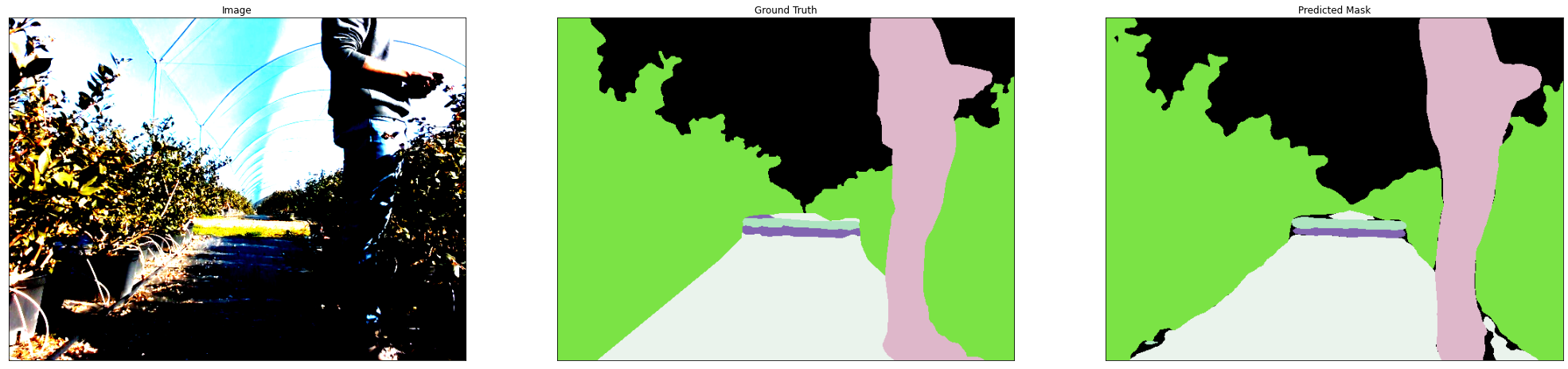
Left: raw image. Middle: ground truth mask. Right: predicted values.

The final results looked very good, and so we felt happy to deliver this to our client.

Final handover

I went out to the farm in Stellenbosch personally to work with the Arcitechnologies team. During the time, I stepped through the code base and model retraining pipeline with them to enable them to enhance the model on their own over time.

This was really valuable time as we got to pressure test the model and see how it performed in reality. To do this, we simply used a laptop with a camera attached and walked it through the blueberry rows. The performance wasn't as good as it had been on the original dataset, but this is something that will improve with more data.

Another consideration that became clear was that the model would run very slowly on the robot, only achieving an FPS of about 1.5. This would not be enough for real-time navigation. However, this can be resolved using techniques like model quantization and potentially through a different architecture.

Reflections and future work

My biggest takeaway from the project was the necessity of testing early to see what the real world requirements are for the model. It would have been much more clear that a big focus on model speed was required if we had done our testing day 2 weeks into the project rather than near the end. This was made difficult by me getting covid halfway into the project, but it was still a powerful learning that I will prioritize in projects going forward.

I think that some other key future work that could help with the client's needs is model quantization which is a great technique for speeding up model performance. This works by reducing the precision of the values that the model works with to make its computations faster without losing much performance. An example would be reducing a 32 length decimal floating point number to an int or float16. This normally has minimal impact because those trailing decimal values do not have a big impact on the models actual predictions and are computationally expensive to handle.

This was a great project, and we especially appreciated the opportunity to share our knowledge of how the training process worked with the client to empower them to build their own models in future. While this was only an early prototype of the model that will be in the final product, the client was convinced that this was the direction to take in solving their autonomous navigation problem.